Data Processing with Matlab
In this page you will find some tips on how to analyze NE instrument data with Matlab. This includes EEG data and accelerometry. In addition, we suggest you to use MATLAB with the EEGLAB toolbox, and the corresponding Plugin for NIC files.
Some basics - working with .easy files

When EEG data is recorded by NIC from Enobio or StarStim instruments, several files are created. These include an .info file and an .easy file. "Easy" format data is, well, easy to load into a program such as Matlab.
See Manuals & Downloads / Repository for more sophisticated sample code to do data analysis. You can find there code to create PSDs plots, spectrograms, etc.
Here is a simple example in Matlab (download the example here). This is a an example file to read NE data. First we load the file - change the filename below as needed. The file should be in the Matlab working directory in this case:
>> d=load(‘20120731153351_enobiodata.easy’);
The data is now loaded as an array in the "d" variable.
You can extract channel locations from the .info file. Here is the list of default Channels for Enobio 20:
LabelsElectrodes={'P7','P4','Cz','Pz','P3','P8','O1','O2','T8','F8',...
       'C4','F4','Fp2','Fz','C3','F3','Fp1','T7','F7','EXT'};
and for Enobio 32:
   LabelsElectrodes={'P7','P4','Cz','Pz','P3','P8','O1','O2',...
       'T8','F8','C4','F4','Fp2','Fz','C3','F3',...
       'Fp1','T7','F7','Oz','PO4','FC6','FC2','AF4', ...
       'CP6','CP2','CP1','CP5','FC1','FC5','AF3','PO3'};
Next we define the time axis using the last column in the data (in ms Unix time):
>> time=d(:,end); % time stamp is in the last column - in ms Unix time
>> time=time-time(1); % set clock to zero in first sample
>> time=time/1000; % change time units to seconds
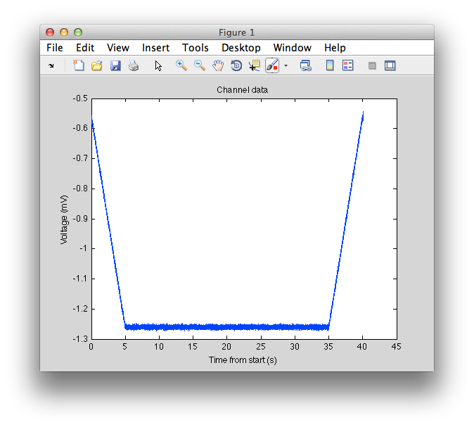
Example 1: we plot channel 1 in mV
>> figure(1); plot(time, d(:,1)/1e6); % divide by one million to go to mV
>> xlabel(‘Time from start (s)’);
>> ylabel(‘Voltage (mV)’);
>> title(‘Channel 1 data’);
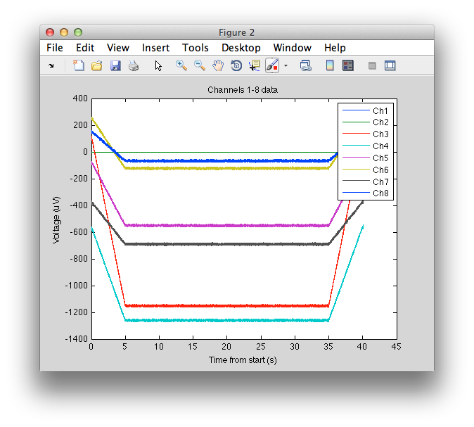
Example 2: we plot channels 1 to 8 in uV
>> figure(2); plot(time, d(:,1:8)/1e3); % divide by one thousand to go to uV
>> xlabel(‘Time from start (s)’);
>> ylabel(‘Voltage (uV)’);
>> legend({‘Ch1’,’Ch2’,’Ch3’,’Ch4’,’Ch5’,’Ch6’,’Ch7’,’Ch8’});
>> title(‘Channels 1-8 data’);
>> ylim([-200 200]); % fix the y-axis limits to plu/minus 200 uV
Using NE_Viewer.m
You can find here a zip file containing the following:
- NE_Viewer.m, a Matlab demo function to read and plot NE files, together with
- CalibrateAccelerometer.m file, a function to calibrate the three axis of the accelerometer.
- some data in .easy format and
- a folder with the figures NE_Viewer.m generates with this data.
The data and code are provided as examples of how to use Matlab to read and plot data.
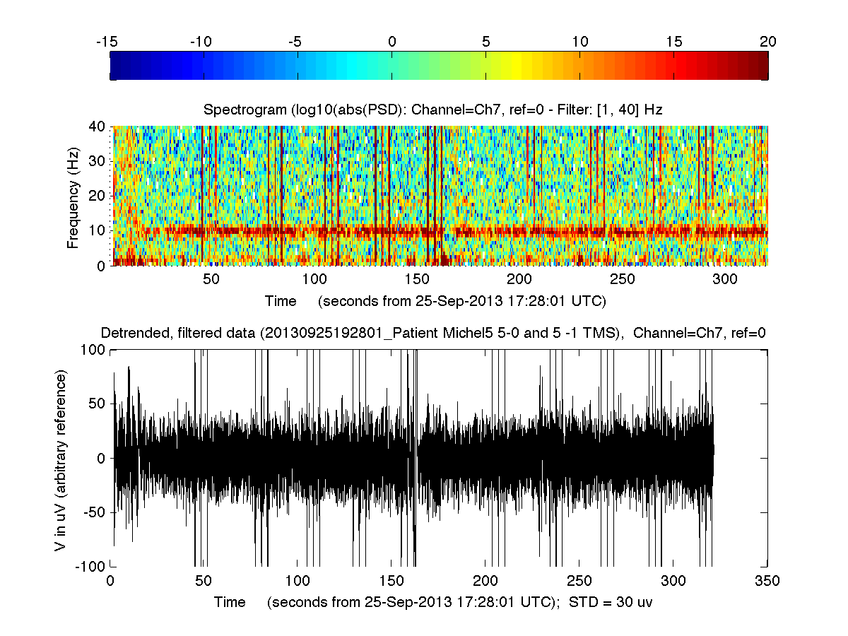
The call used to generate the plots in the folder is
>> NE_Viewer('20130925192801_PatientTMS.easy',999,500,{'Fp1','Fp2','F3','F4','C3','C4','P3','Cz'});
The 999 mean "do average referencing" and the 500 is the sampling rate in S/s. The rest are electrode labels (the data has been collected using a StarStim 8 channels system).
Here is the header of NE_Viewer:
function [NEdata NEdataRefFilPack]= ...
                     NE_Viewer(filepath, ref, fs, LabelsElectrodes,band,T)
% NE_Viewer(filepath) reads Enobio/StarStim (3G, released 2012) data in
% ASCII (.txt or ".easy") or EDF format, and plots parts of it together
% with its PSD and spectrogram.
%
% This function is provided as is as an example on how to work with NE instrument
% data.
%
% INPUTS:
% Enobio/StarStim (8 or 20 or 32 Ch) data file path (mandatory) and other optional
% entries: "ref" the optional reference channel (use 0 for none, 999 for
% an all electrode average), "fs" the sampling rate in S/s,
% "LabelsElectrodes" a structure containing channel names, and "band" a
% 2-element array with the low and high filtering frequency, e.g.,
% band=[1 40], in Hz. Finally, "T" is an arracy specifiying initital and
% final time to analyze (in seconds), e.g., T=[10 130].
%
% OUTPUTS:
% Returns the original, raw data pack, NEdata, as a Matlab variable.
% preserving the units (e.g., nV, ms). It also returnes NEdataRefFilPack,
% the processed (referenced, detreneded, filtered) data (in uV). The time
% stamp (in seconds from start of the take) is provided in the last column.
%
% SIDE EFFECTS: creation of "figures" directory if it does not exist,
%               creation of data plot figures of all Enobio channels, etc.
%
%       out = NE_Viewer(filepath) plots the data in the filepath
%       (filepath includes path relative to the Matlab current working
%       directory of full absolute path), its PSD and spectrogram for each channel,
%       etc., for 8 channels. As default it assumes a 500 Samples/s
%       sampling rate, and does not reference the data to any other
%       channel.  The code puts figures in a directory under the working
%       directory.
%
%       NE_Viewer(filepath, ref) references the data to a chosen channel
%       (ref should be a Channel number from 1 to 8 (or 20 for Enobio20),
%       or zero to force no reference - the default). A reference = 999
%       means the average of all electrodes is used as reference.
%
%       In addition, using the call NE_View(filepath, ref, fs) allows
%       for changing the sampling rate fs in Samples/s.
%
%       Use a structure with LabelsElectrodes such as
%         >> LabelsElectrodes={'Ch1','Ch2','Ch3','Ch4','Ch5','Ch6','Ch7','Ch8'}
%       with
%         >> NE_View(filepath, ref, fs, LabelsElectrodes)
%       to add LabelsElectrodes to channel IDs in plots.
%
%
% EXAMPLE: assuming the data is in a folder called "data",
%          NE_Viewer('./data/EC.txt')   % uses all defaults
%          NE_Viewer('./data/EC.txt',1)    % spedifies reference channel
%          NE_Viewer('./data/EC.txt',1,500) % specifies Sampling rate
%
%          To specify channel LabelsElectrodes
%          NE_Viewer('./data/EC.txt',1,500, ...
%                    {'Fp1','Fp2','P3','P4','O1','O1','T7','Pz'} )
%
%          To specifiy a filter band other than the default:
%          NE_Viewer('data/StarStim/20120728085042_TBtACS10Hz1mA.txt',0, ...
%                                                         [],[],[1 60]);
%
%    As another example,
%
%       >> [NEdata NEdataRefFilPack]=NE_Viewer('data/Enobio8.txt');
%   and then plot data vs. time
%       >> figure; plot(NEdataRefFilPack(:,9), NEdataRefFilPack(:,1));
%
% ABOUT THE NE ASCII DATA FORMAT (July 2012):
%       NE ASCII files contain one line per time sample. Each line contains
%       first the EEG data (8 or 20 channels, depending on the device, with
%       units in nV), followed by  three acceleration channels (aX,aY,aZ
%       in mm/s^2- millimeters per second squared), an *optional* external
%       input channel, a trigger flag (int32) and, finally,
%       a timestamp in Unix time (ms from Jan 1 1970):
%
% Ch1(nV) ... Ch8or20(nV) aX(mg) aY(mg) aZ(mg) AddSensor Flags(uint32) TimeStamp (ms)
%
% Therefore Enobio8/StarStim will have a minimum of 8+2 (10) columns, or 8+3=11 if no
%   accelerometer or >= 8+4 (with accelerometer). In summary:
%
%   Enobio8/20
%        10 Columns: no AddSensor, no accelerometer data:
%        11 Comumns: no accelerometer, but there is AddSensor
%        13 Columns: there is accelerometer, but no Addsensor
%        14 Comumns: there is accelerometer, AddSensor.
%
%   Enobio 20 will have >= 22 and >=24 columns if acc. data present:
%        22 Columns: no AddSensor, no accelerometer
%        23 Comumns: no accelerometer, but there is AddSensor
%        25 Columns: there is accelerometer, no AddSensor
%        26 Comumns: there is accelerometer, AddSensor.
%
%   Enobio 32 will have >=34 adn >=36 if acc data is present
%        34 Columns: no AddSensor, no accelerometer
%        35 Comumns: no accelerometer, but there is AddSensor
%        37 Columns: there is accelerometer, no AddSensor
%        38 Comumns: there is accelerometer, AddSensor.
%
%   Author(s): G.R. - Neuroelectrics Barcelona SL
%   Copyright 2011-13 Neuroelectrics Barcelona SL
%   $Revision: 0.1 $  $Date: 2011/11/26 $
%   $Revision: 0.2 $  $Date: 2012/07/16 $
%   $Revision: 0.3 $  $Date: 2012/11/15 $
%   $Revision: 0.4 $  $Date: 2013/01/11 $
%   $Revision: 1.0 $  $Date: 2013/01/15 $
%   $Revision: 1.1 $  $Date: 2013/01/15 $

%   References:
%     [1] Enobio users guide. http://neuroelectrics.com

